Marker-less Augmented Reality by OpenCV and OpenGL
In this project readers will learn how to create a standard real-time project using OpenCV (for desktop), and how to perform a new method of marker-less augmented reality, using the actual environment as the input instead of printed square markers. This project covers some of the theory of marker-less AR and show how to apply it in useful projects.
You can find more information about the source code at GitHub.
Quick Demo


What is Augmented Reality?
Augmented reality may be defined as reality created with the help of additional computer elements. Among famous examples are arrows pointing at the distance from the penalty kick to the woodwork, mixing real and fictional objects in movies, computer and gadget games etc.
In other words,augmented reality (AR) is a view of things of real world enriched (augmented) by video, GPS, graphics or sound. This technology helps to enhance human perception of reality, it is happening in a real time in a definite context.

The biggest advantage of Augmented Reality is the bridge that is gapped between the digital and real worlds. The promotion and marketing of products from interactive games to 3D experiences are offered on a whole new level through our exceptional options. Our Mobile Augmented Reality applications are rapidly growing in popularity, due to its easy downloadable features and dynamic uses on any smart phone.
Solutions include GPS or geolocation to blending contextual information in any situation by way of the applications. The combination of these two separate technologies, enable Augmented Reality applications to go mainstream and bring users a variety of truly immersive experiences.
1. INRODUCTION
A marker is usually designed as a rectangle image holding black and white areas inside it. Due to known limitations, the marker detection procedure is a simple one. First of all we need to find closed contours on the input image and unwarp the image inside it to a rectangle and then check this against our marker model.
For example, the 5 x 5 marker looks like:

The strong aspects of the markers are as follows:
- Cheap detection algorithm
- Robust against lighting changes
Markers also have several weaknesses. They are as follows:
- Doesn’t work if partially overlapped
- Marker image has to be black and white
- Has square form in most cases (because it’s easy to detect)
- Non-esthetic visual look of the marker
- Has nothing in common with real-world objects
So, markers are a good point to start working with augmented reality; but if you want more, it’s time to move on from marker-based to marker-less AR. Marker-less AR is a technique that is based on recognition of objects that exist in the real world. A few examples of a target for marker-less AR are: magazine covers, company logos, toys, and so on. In general, any object that has enough descriptive and discriminative information regarding the rest of the scene can be a target for marker-less AR.
The strong sides of the marker-less AR approach are:
- Can be used to detect real-world objects
- Works even if the target object is partially overlapped
- Can have arbitrary form and texture (except solid or smooth gradient textures)
Marker-less AR systems can use real images and objects to position the camera in 3D space and present eye-catching effects on top of the real picture. The heart of the marker-less AR are image recognition and object detection algorithms. Unlike markers, whose shape and internal structure is fixed and known, real objects cannot be defined in such a way. Also, objects can have a complex shape and require modified pose estimation algorithms to find their correct 3D transformations.
Marker-less AR performs heavy CPU calculations, so a mobile device often is not capable to secure smooth FPS. In this project, we will be targeting desktop platforms such as PC or Mac. For this purpose, we need a cross-platform build system. In this project we use the CMake build system.
Before we start, let me give you a brief list of the knowledge required for this project and the software you will need:
- Basic knowledge of CMake. CMake is a cross-platform, open-source build system designed to build, test, and package software. Like the OpenCV library, the demonstration project for this chapter also uses the CMake build system. CMake can be downloaded from here.
- A basic knowledge of C++ programming language is also necessary.

2. THEORY
- ) MarkerlessAR_V1: It is the first version of “Open Source Markerless Augmented Reality” and it has the capabilities which is listed at below.
a.) Using Feature Descriptors to Find an Arbitrary Image on Video
In this project, I am interested in corner detection. The corner detection is based on an analysis of the edges in the image. A corner-based edge detection algorithm searches for rapid changes in the image gradient. Usually it’s done by looking for extremums of the first derivative of the image gradients in the X and Y directions.
b.) Feature Extraction
OpenCV has several feature-detection algorithms. All of them are derived from the base class cv::FeatureDetector. Creation of the feature-detection algorithm can be done in two ways:
- Via an explicit call of the concrete feature detector class constructor:
cv::Ptrcv::FeatureDetector detector = cv::Ptrcv::FeatureDetector(new cv::SurfFeatureDetector());- Or by creating a feature detector by algorithm name:
cv::Ptrcv::FeatureDetector detector = cv::FeatureDetector::create(“SURF”);Both methods have their advantages, so choose the one you most prefer. The explicit class creation allows you to pass additional arguments to the feature detector constructor, while the creation by algorithm name makes it easier to switch the algorithm during runtime. To detect feature points, you should call the detect method:
std::vector<cv::KeyPoint> keypoints;
detector->detect(image, keypoints);
If we deal with images, which usually have a color depth of 24 bits per pixel, for a resolution of 640 x 480, we have 912 KB of data. How do we find our pattern image in the real world? Pixel-to-pixel matching takes too long and we will have to deal with rotation and scaling too. It’s definitely not an option. Using feature points can solve this problem. By detecting keypoints, we can be sure that returned features describe parts of the image that contains lot of information (that’s because corner-based detectors return edges, corners, and other sharp figures). So to find correspondences between two frames, we only have to match keypoints.
From the patch defined by the keypoint, we extract a vector called descriptor. It’s a form of representation of the feature point. There are many methods of extraction of the descriptor from the feature point. All of them have their strengths and weaknesses. For example, SIFT and SURF descriptor-extraction algorithms are CPU-intensive but provide robust descriptors with good distinctiveness. In our sample project we use the ORB descriptor-extraction algorithm because we choose it as a feature detector too.
It’s always a good idea to use both feature detector and descriptor extractor from the same algorithm, as they will then fit each other perfectly.
Feature descriptor is represented as a vector of fixed size (16 or more elements). Let’s say our image has a resolution of 640 x 480 pixels and it has 1,500 feature points. Then, it will require 1500 * 16 * sizeof(float) = 96 KB (for SURF). It’s ten times smaller than the original image data. Also, it’s much easier to operate with descriptors rather than with raster bitmaps. For two feature descriptors we can introduce a similarity score — a metric that defines the level of similarity between two vectors. Usually its L2 norm or hamming distance (based upon the kind of feature descriptor used).
c.) Definition of a Pattern Object
To describe a pattern object we introduce a class called Pattern, which holds a train image, list of features and extracted descriptors, and 2D and 3D correspondences for initial pattern position:
/**
* Store the image data and computed descriptors of target pattern
*/
struct Pattern {

    cv::Size size;
    cv::Mat data;
    std::vector<cv::KeyPoint> keypoints;
    cv::Mat descriptors;
    std::vector<cv::Point2f> points2d;
    std::vector<cv::Point3f> points3d;

};
d.) Matching of Feature Points
The process of finding frame-to-frame correspondences can be formulated as the search of the nearest neighbor from one set of descriptors for every element of another set. It’s called the “matching” procedure.
The following code block trains the descriptor matcher using the pattern image PatternDetector.cpp:
void PatternDetector::train(const Pattern& pattern) {

    // Store the pattern object
    m_pattern = pattern;

    // API of cv::DescriptorMatcher is somewhat tricky
    // First we clear old train data:
    m_matcher->clear();

    // That we add vector of descriptors
    // (each descriptors matrix describe one image).
    // This allows us to perform search across multiple images:
    std::vector<cv::Mat> descriptors(1);
    descriptors[0] = pattern.descriptors.clone();
    m_matcher->add(descriptors);

    // After adding train data perform actual train:
    m_matcher->train();}
To match query descriptors, we can use one of the following methods of cv::DescriptorMatcher:
- To find the simple list of best matches:
void match(const Mat& queryDescriptors, vector& matches, const vector& masks=vector() );- To find K nearest matches for each descriptor:
void knnMatch(const Mat& queryDescriptors, vector<vector >& matches, int k, const vector& masks=vector ), bool compactResult=false );- To find correspondences whose distances are not farther than the specified distance:
void radiusMatch(const Mat& queryDescriptors, vector<vector >& matches, maxDistance, const vector& masks=vector(), bool compactResult=false );d.) Outlier Removal
Mismatches during the matching stage can happen. It’s normal. There are two kinds of errors in matching:
- False-positive matches: When the feature-point correspondence is wrong
- False-negative matches: The absence of a match when the feature points are visible on both images
False-negative matches are obviously bad. But we can’t deal with them because the matching algorithm has rejected them. Our goal is therefore to minimize the number of false-positive matches. To reject wrong correspondences, we can use a cross-match technique. The idea is to match train descriptors with the query set and vice versa. Only common matches for these two matches are returned. Such techniques usually produce best results with minimal number of outliers when there are enough matches.

The well-known outlier-removal technique is the ratio test. We perform KNN-matching first with K=2. Two nearest descriptors are returned for each match. The match is returned only if the distance ratio between the first and second matches is big enough (the ratio threshold is usually near two).
The following code performs robust descriptor matching using a ratio test PatternDetector.cpp:
void PatternDetector::getMatches(const cv::Mat& queryDescriptors, std::vector<cv::DMatch>& matches) {

    matches.clear();
    if (enableRatioTest) {

        // To avoid NaNs when best match has
        // zero distance we will use inverse ratio.
        const float minRatio = 1.f / 1.5f;

        // KNN match will return 2 nearest
        // matches for each query descriptor
        m_matcher->knnMatch(queryDescriptors, m_knnMatches, 2);

        for (size_t i=0; i<m_knnMatches.size(); i++) {

            const cv::DMatch& bestMatch = m_knnMatches[i][0];
            const cv::DMatch& betterMatch = m_knnMatches[i][1];
            float distanceRatio = bestMatch.distance /
            betterMatch.distance;            // Pass only matches where distance ratio between
            // nearest matches is greater than 1.5
            // (distinct criteria)
            if (distanceRatio < minRatio) {

                matches.push_back(bestMatch);

            }

        }

    }    else {        // Perform regular match
        m_matcher->match(queryDescriptors, matches);    }
}
The ratio test can remove almost all outliers. But in some cases, false-positive matches can pass through this test. In the next section, we will show you how to remove the rest of outliers and leave only correct matches.
e.) Homography Estimation
To improve our matching even more, we can perform outlier filtration using the random sample consensus (RANSAC) method. As we’re working with an image (a planar object) and we expect it to be rigid, it’s ok to find the homography transformation between feature points on the pattern image and feature points on the query image. Homography transformations will bring points from a pattern to the query image coordinate system.
See this interesting paper for more information deeply about Homography Estimation.
The paper describes a method to filter out some wrong correspondences before computing homographies in the RANSAC algorithm.
The following code which is located in PatternDetector.cpp uses a homography matrix estimation using a RANSAC algorithm to filter out geometrically incorrect matches:
bool PatternDetector::refineMatchesWithHomography(const std::vector<cv::KeyPoint>& queryKeypoints, const std::vector<cv::KeyPoint>& trainKeypoints, float reprojectionThreshold, std::vector<cv::DMatch>& matches, cv::Mat& homography ) {    const int minNumberMatchesAllowed = 8;

    if (matches.size() < minNumberMatchesAllowed)
        return false;

    // Prepare data for cv::findHomography
    std::vector<cv::Point2f> srcPoints(matches.size());
    std::vector<cv::Point2f> dstPoints(matches.size());
    for (size_t i = 0; i < matches.size(); i++) {

        srcPoints[i] = trainKeypoints[matches[i].trainIdx].pt;
        dstPoints[i] = queryKeypoints[matches[i].queryIdx].pt;

    }

    // Find homography matrix and get inliers mask
    std::vector<unsigned char> inliersMask(srcPoints.size());
    homography = cv::findHomography(srcPoints,
    dstPoints,
    CV_FM_RANSAC,
    reprojectionThreshold,
    inliersMask);
    std::vector<cv::DMatch> inliers;
    for (size_t i=0; i<inliersMask.size(); i++) {

        if (inliersMask[i])
            inliers.push_back(matches[i]);

    }

    matches.swap(inliers);
    return matches.size() > minNumberMatchesAllowed;}
f.) Homography Refinement
When we look for homography transformations, we already have all the necessary data to find their locations in 3D. However, we can improve its position even more by finding more accurate pattern corners. For this we warp the input image using estimated homography to obtain a pattern that has been found. The result should be very close to the source train image. Homography refinement can help to find more accurate homography transformations.
The following code block contains the final version of the pattern detection routine which is located in PatternDetector.cpp;
bool PatternDetector::findPattern(const cv::Mat& image, PatternTrackingInfo& info) {    // Convert input image to gray
    getGray(image, m_grayImg);

    // Extract feature points from input gray image
    extractFeatures(m_grayImg, m_queryKeypoints,
    m_queryDescriptors);

    // Get matches with current pattern
    getMatches(m_queryDescriptors, m_matches);

    // Find homography transformation and detect good matches
    bool homographyFound = refineMatchesWithHomography(
    m_queryKeypoints,
    m_pattern.keypoints,
    homographyReprojectionThreshold,
    m_matches,
    m_roughHomography);

    if (homographyFound) {

        // If homography refinement enabled
        // improve found transformation
        if (enableHomographyRefinement) {

            // Warp image using found homography
            cv::warpPerspective(m_grayImg, m_warpedImg,
            m_roughHomography, m_pattern.size,
            cv::WARP_INVERSE_MAP | cv::INTER_CUBIC);

            // Get refined matches:
            std::vector<cv::KeyPoint> warpedKeypoints;
            std::vector<cv::DMatch> refinedMatches;

            // Detect features on warped image
            extractFeatures(m_warpedImg, warpedKeypoints,
            m_queryDescriptors);

            // Match with pattern
            getMatches(m_queryDescriptors, refinedMatches);

            // Estimate new refinement homography
            homographyFound = refineMatchesWithHomography(
            warpedKeypoints,
            m_pattern.keypoints,
            homographyReprojectionThreshold,
            refinedMatches,
            m_refinedHomography);

            // Get a result homography as result of matrix product
            // of refined and rough homographies:
            info.homography = m_roughHomography *
            m_refinedHomography;

            // Transform contour with precise homography
            cv::perspectiveTransform(m_pattern.points2d,
            info.points2d, info.homography);

        }

        else {

        info.homography = m_roughHomography;

        // Transform contour with rough homography
        cv::perspectiveTransform(m_pattern.points2d,
        info.points2d, m_roughHomography);

        }
    }

    return homographyFound;

}
If, after all the outlier removal stages, the number of matches is still reasonably large (at least 25 percent of features from the pattern image have correspondences with the input one), you can be sure the pattern image is located correctly. If so, we proceed to the next stage — estimation of the 3D position of the pattern pose with regards to the camera.
Let’s conclude again with a brief list of the steps we performed:
- Converted input image to grayscale.
- Detected features on the query image using our feature-detection algorithm.
- Extracted descriptors from the input image for the detected feature points.
- Matched descriptors against pattern descriptors.
- Used cross-checks or ratio tests to remove outliers.
- Found the homography transformation using inlier matches.
- Refined the homography by warping the query image with homography from the previous step.
- Found the precise homography as a result of the multiplication of rough and refined homography.
- Transformed the pattern corners to an image coordinate system to get pattern locations on the input image.
g.) Pattern pose estimation
The pose estimation is done in a similar manner to marker pose estimation from the previous chapter. As usual we need 2D-3D correspondences to estimate the camera-extrinsic parameters. We assign four 3D points to coordinate with the corners of the unit rectangle that lies in the XY plane (the Z axis is up), and 2D points correspond to the corners of the image bitmap.
The are 2D-3D correspondences are given at the below. Camera pose estimation allows to place objects in the scene.

The buildPatternFromImage class creates a Pattern object from the input image as follows:
void PatternDetector::buildPatternFromImage(const cv::Mat& image, Pattern& pattern) const {    int numImages = 4;    float step = sqrtf(2.0f);    // Store original image in pattern structure
    pattern.size = cv::Size(image.cols, image.rows);
    pattern.frame = image.clone();
    getGray(image, pattern.grayImg);    // Build 2d and 3d contours (3d contour lie in XY plane since
    // it's planar)
    pattern.points2d.resize(4);
    pattern.points3d.resize(4);    // Image dimensions
    const float w = image.cols;
    const float h = image.rows;    // Normalized dimensions:
    const float maxSize = std::max(w,h);
    const float unitW = w / maxSize;
    const float unitH = h / maxSize;    pattern.points2d[0] = cv::Point2f(0,0);
    pattern.points2d[1] = cv::Point2f(w,0);
    pattern.points2d[2] = cv::Point2f(w,h);
    pattern.points2d[3] = cv::Point2f(0,h);
    pattern.points3d[0] = cv::Point3f(-unitW, -unitH, 0);
    pattern.points3d[1] = cv::Point3f( unitW, -unitH, 0);
    pattern.points3d[2] = cv::Point3f( unitW, unitH, 0);
    pattern.points3d[3] = cv::Point3f(-unitW, unitH, 0);    extractFeatures(pattern.grayImg, pattern.keypoints,pattern.descriptors);}
This configuration of corners is useful as this pattern coordinate system will be placed directly in the center of the pattern location lying in the XY plane, with the Z axis looking in the direction of the camera.
h.) Rendering Augmented Reality (without 3D model parsing just with OpenGL draw functions)
I introduce the ARDrawingContext.cpp structure to hold all the necessary data that visualization may need:
- The most recent image taken from the camera
- The camera-calibration matrix
- The pattern pose in 3D (if present)
- The internal data related to OpenGL (texture ID and so on)
i.) Application Infrastructure
So far, we’ve learned how to detect a pattern and estimate its 3D position with regards to the camera. Now it’s time to show how to put these algorithms into a real application. So our goal for this section is to show how to use OpenCV to capture a video from a web camera and create the visualization context for 3D rendering. As our goal is to show how to use key features of marker-less AR, we will create a simple command-line application that will be capable of detecting arbitrary pattern images either in a video sequence or in still images.

It consists of:
- The camera-calibration object
- An Instance of the pattern-detector object
- A trained pattern object
- Intermediate data of pattern tracking
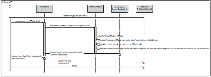
Almost all things are done. We create a pattern-detection algorithm and then we estimate the pose of the found pattern in 3D space, a visualization system to render the AR. Let’s take a look at the following UML sequence diagram that demonstrates the frame-processing routine in our app:
k.) Demonstration
- The Demo video of this step is available on Youtube: https://www.youtube.com/watch?v=caWl8nG6mLk
- The screenshot:

2.) MarkerlessAR_V2: It is the second version of “Open Source Markerless Augmented Reality” and it has the capabilities which are listed at below.
a.) Parsing the 3D(OBJ) Model
Example OBJ File
mtllib cube.mtl
v 1.000000 -1.000000 -1.000000
v 1.000000 -1.000000 1.000000
v -1.000000 -1.000000 1.000000
v -1.000000 -1.000000 -1.000000
v 1.000000 1.000000 -1.000000
v 0.999999 1.000000 1.000001
v -1.000000 1.000000 1.000000
v -1.000000 1.000000 -1.000000
vt 0.748573 0.750412
vt 0.749279 0.501284
vt 0.999110 0.501077
vt 0.999455 0.750380
vt 0.250471 0.500702
vt 0.249682 0.749677
vt 0.001085 0.750380
vt 0.001517 0.499994
vt 0.499422 0.500239
vt 0.500149 0.750166
vt 0.748355 0.998230
vt 0.500193 0.998728
vt 0.498993 0.250415
vt 0.748953 0.250920
vn 0.000000 0.000000 -1.000000
vn -1.000000 -0.000000 -0.000000
vn -0.000000 -0.000000 1.000000
vn -0.000001 0.000000 1.000000
vn 1.000000 -0.000000 0.000000
vn 1.000000 0.000000 0.000001
vn 0.000000 1.000000 -0.000000
vn -0.000000 -1.000000 0.000000
usemtl Material_ray.png
s off
f 5/1/1 1/2/1 4/3/1
f 5/1/1 4/3/1 8/4/1
f 3/5/2 7/6/2 8/7/2
f 3/5/2 8/7/2 4/8/2
f 2/9/3 6/10/3 3/5/3
f 6/10/4 7/6/4 3/5/4
f 1/2/5 5/1/5 2/9/5
f 5/1/6 6/10/6 2/9/6
f 5/1/7 8/11/7 6/10/7
f 8/11/7 7/12/7 6/10/7
f 1/2/8 2/9/8 3/13/8
f 1/2/8 3/13/8 4/14/8
So :
- usemtl and mtllib describe the look of the model. We won’t use this in this tutorial.
- v is a vertex
- vt is the texture coordinate of one vertex
- vn is the normal of one vertex
- f is a face
v, vt and vn are simple to understand. f is more tricky. So, for f 8/11/7 7/12/7 6/10/7 :
- 8/11/7 describes the first vertex of the triangle
- 7/12/7 describes the second vertex of the triangle
- 6/10/7 describes the third vertex of the triangle (duh)
- For the first vertex, 8 says which vertex to use. So in this case, -1.000000 1.000000 -1.000000 (index start to 1, not to 0 like in C++)
- 11 says which texture coordinate to use. So in this case, 0.748355 0.998230
- 7 says which normal to use. So in this case, 0.000000 1.000000 -0.000000
These numbers are called indices. It’s handy because if several vertices share the same position, you just have to write one “v” in the file, and use it several times. This saves memory.
The bad news is that OpenGL can’t be told to use one index for the position, another for the texture, and another for the normal.
As you can get it from above that the OBJ files just includes vertices, texture coordinates and normals. If we want to render/load 3D OBJ model, we should parse the OBJ file so we will get the vertices, texture coordinates and normals. Here is the obj parser. By using it, you can parse the OBJ files to get the vertices, texture coordinates and normals.
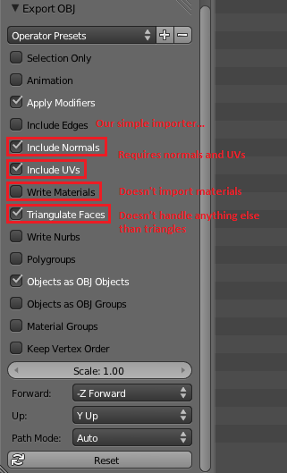
Since our toy loader is severely limited, we have to be extra careful to set the right options when exporting the file. Here’s how it should look in Blender :
b.) Loading / Rendering the 3D model
After getting the vertices, texture coordinates and normals by using OBJ parser, you can use “glNormal3f(x, y, z)”, “glTexCoord2d(x, y)” and “glVertex3f(x, y, z)” for rendering 3D model by OpenGL. This is the sample method which is located in ARDrawingContext.cpp;
void ARDrawingContext::draw3DModel() { // a method to render 3D model by using OpenGL    glEnable(GL_TEXTURE_2D); // enable server-side GL capabilities
    glBindTexture(GL_TEXTURE_2D, Texture); //
    glBegin(GL_TRIANGLES); // delimit the vertices of a primitive or a group of like primitives

    for (int i = 0; i < vertices.size(); i += 1) { // for loop to cover all vertices, normals and texture coordinates        a = vertices[i];
        b = uvs[i];
        glNormal3f(a.x, a.y, a.z); // it renders the "normals"
        glTexCoord2d(b.x, b.y); // it renders the "texture"
        glVertex3f(a.x, a.y, a.z); // it renders the "vertices"    }    glEnd(); //end drawing of line loop
    glDisable(GL_TEXTURE_2D); // disable server-side GL capabilities}
c.) Scaling the 3D model
All vertex, normal and texture points should be multiplied by scale factor to scale the 3D model. This is he sample method which is located in ARDrawingContext.cpp;
void ARDrawingContext::scale3DModel(float scaleFactor) {    for (int i = 0; i < vertices.size(); i += 1) {

        // multiplying vertices by scale factor to scale 3d model
        vertices[i] = vertices[i] * vec3(scaleFactor * 1.0f, scaleFactor * 1.0f, scaleFactor * 1.0f);

    }    for (int i = 0; i < normals.size(); i += 1) {

        // multiplying normals by scale factor to scale 3d model
        normals[i] = normals[i] * vec3(scaleFactor * 1.0f, scaleFactor * 1.0f, scaleFactor * 1.0f);

    }    for (int i = 0; i < uvs.size(); i += 1) {

        // multiplying faces by scale factor to scale 3d model
        uvs[i] = uvs[i] * vec2(scaleFactor * 1.0f, scaleFactor * 1.0f);

    }

}
d.) Loading .BMP File as a Texture to on 3D model
See texture.cpp for more information.
e.) UV Mapping (projecting a 2D image to a 3D model’s surface for texture mapping)
UV mapping is the 3D modeling process of projecting a 2D image to a 3D model’s surface for texture mapping.
This process projects a texture map onto a 3D object. The letters “U” and “V” denote the axes of the 2D texture because “X”, “Y” and “Z” are already used to denote the axes of the 3D object in model space.
UV texturing permits polygons that make up a 3D object to be painted with color (and other surface attributes) from an ordinary image. The image is called a UV texture map.The UV mapping process involves assigning pixels in the image to surface mappings on the polygon, usually done by “programmatically” copying a triangular piece of the image map and pasting it onto a triangle on the object.[2] UV is an alternative to projection mapping (e.g. using any pair of the model’s X,Y,Z coordinates, or any transformation of the position); it only maps into a texture space rather than into the geometric space of the object. But the rendering computation uses the UV texture coordinates to determine how to paint the three-dimensional surface.
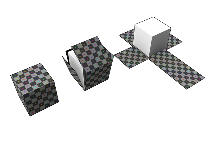
A representation of the UV mapping of a cube. The flattened cube net may then be textured to texture the cube;
See texture.cpp for more information.
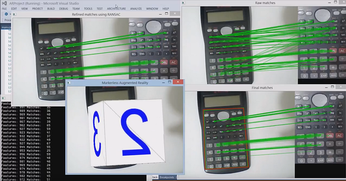
f.) Demonstration
- The Demo video of this step is available on Youtube: https://www.youtube.com/watch?v=nPfR5ACrqu0
- The screenshot:
3. INSTALLATION
To build this app use the CMake to generate project files for your IDE, then build the project in your IDE.
NOTE: You will need to have OpenCV built with OpenGL support in order to run the demo (prebuilt versions of OpenCV don’t support OpenGL).
How to enable OpenGL Support in OpenCV:
- Linux: Execute;
sudo apt-get install libgtkglext1 libgtkglext1-dev
- MacOSX: Install QT4 and then configure OpenCV with QT and OpenGL.
- Windows: Enable WITH_OPENGL=YES flag when building OpenCV to enable OpenGL support.
Building the project using CMake from the command-line:
- Linux:
export OpenCV_DIR="~/OpenCV/build"
mkdir build
cd build
cmake -D OpenCV_DIR=$OpenCV_DIR ..
make- MacOSX (Xcode):
export OpenCV_DIR="~/OpenCV/build"
mkdir build
cd build
cmake -G Xcode -D OpenCV_DIR=$OpenCV_DIR ..
open ARProject.xcodepro
Running the project:
Just execute “ARProject”.
4. USAGE
- To run on a single image call:
- ARProject pattern.png test_image.png- To run on a recorded video call:
- ARProject pattern.png test_video.avi- To run using live feed from a web camera, call:
- ARProject pattern.png5. FUTURE WORKS
These 2 important tasks are in progress and they will be submitted with MarkerlessAR_V3 soon:
- IN PROGRESS: Working on Performance Issues to Get Realtime Tracking by using Dimension Reduction which is the process of reducing the number of random variables under consideration, via obtaining a set of principal variables.
- TO DO: Multiple Object Detection And Tracking
6. CITATION
.@ONLINE{vdtc,
      author = "Ahmet Özlü",
      title  = "Open Source Markerless Augmented Reality",
      year   = "2017",
      url    = "https://github.com/ahmetozlu/open_source_markerless_augmented_reality"
  }
7. AUTHOR
Ahmet Özlü
8. LICENSE
This system is available under the MIT license. See the LICENSE file for more info.
9. SUMMARY
In the first version of the project you have learned about feature descriptors and how to use them to define a scale and a rotation invariant pattern description. This description can be used to find similar entries in other images. The strengths and weaknesses of most popular feature descriptors were also explained. Moreover, we learned how to use OpenGL and OpenCV together for rendering augmented reality.
In the second version of the project, parsing, rendering and scaling 3D (OBJ) model was learned. UV mapping and some texture operations also was learned.
